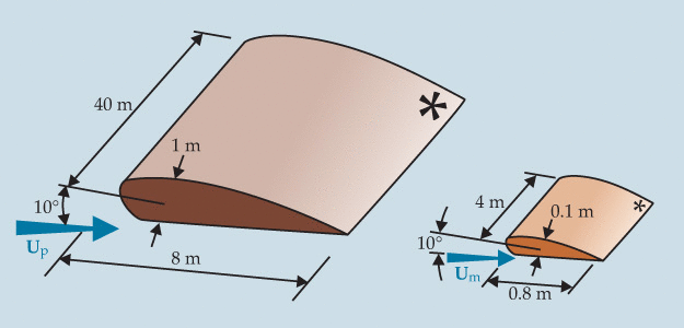
What is Similarity Law Fluid Mechanics?

Table of Contents

Similarity laws are concepts applicable to test engineering models. A model is said to have similarity with the actual case if the two have geometric similarity, kinematic similarity, and dynamic similarity. Sometimes, instead of similarity, similitude can be used. The term dynamic similarity implies that geometric and kinematic similarities are satisfied.

The main application of similarity is in hydraulic and aerospace engineering to study fluid flow conditions with scaled models. In addition, in many textbooks in fluid mechanics, similarity is a primary theory to derive formulas from.

For example, similarity laws provide an excellent tool for classifying turbopumps in the same families. This classification helps designers to engineer similar pumps with the same information. It also provides a useful tool for turbomachinery users to choose the best machine for their application and modify them to suit specific conditions.

The concept of similarity laws is strongly attached to dimensional analysis.

Conceptual Basics of Similarity

Engineering models can be made to study difficult fluid dynamics problems in which calculations and computer simulations are unreliable. Models are often smaller than the actual design, but not always. Scaled models allow a design to be pre-fabricated, and in many cases, are essential steps in the development process.

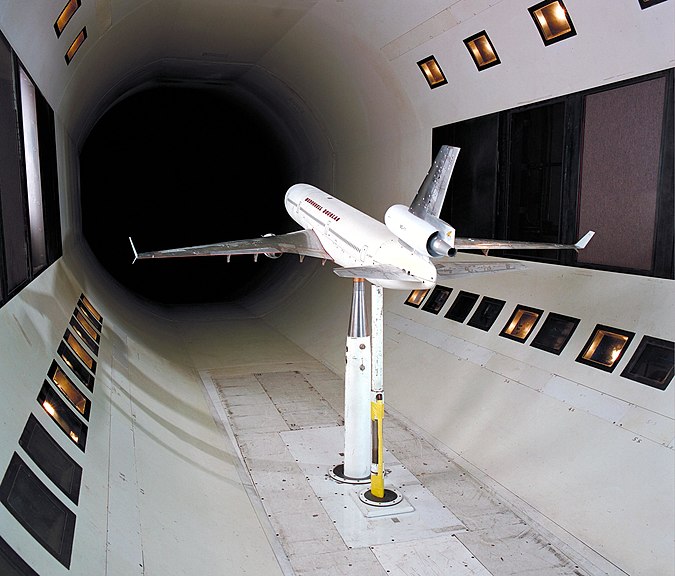
similarity laws — A scaled model for testing an airplane inside a wind tunnel (Reference: **en.wikiversity.org**)

However, the construction of a scaled model must be conducted along with an analysis to determine under what conditions it is tested. While the geometry of the actual model may be easily scaled, other parameters, including pressure, temperature, velocity, and type of fluid, may need to be changed. The similarity is achieved when the test conditions are created in such a way that the test outcomes are applicable to the real model.

To have a similar scaled model to the real case, the following criteria must be met:

Geometric Similarity

The scaled model has the same shape as the application. More precisely, the model can be obtained from the actual case with a uniform scaling (enlarging or reducing).

For example, all circles are geometrically similar to each other. The same goes for all squares and all equilateral triangles. On the other hand, ellipses are not all similar to each other, as well as all rectangles and even isosceles triangles. If the two angles of a triangle are equal to the two angles of another triangle, these triangles are similar to each other.

Kinematic Similarity

Kinematic similarity means that the velocity at any point in the flow of the model is proportional to the velocity at the homologous point in the prototype by a constant scale factor. Thus, it maintains the same flow streamline pattern. This is a necessary condition for complete similarities between the model and the prototype. In other words, the kinematic similarity refers to the similarity of motion of the fluid. As motions can be expressed in terms of distance and time, it means the similarity of lengths (geometrical similarity) and the time intervals similarity.

To obtain kinematic similarity in a scaled model, dimensionless groups are considered the field of fluid dynamics. For example, in many analyses, the Reynolds number of the model and the prototype must be equal. There are other dimensionless numbers to consider, which we will discuss in more detail in the following sections.

Dynamic Similarity

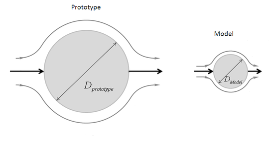
In the field of fluid mechanics, dynamic similarity means that when there are two geometrically similar items with the same shapes and different sizes, the same boundary conditions, and equal dimensionless numbers, then the fluid flows will be the same. From examining the basic Navier-Stokes equation, with geometrically similar bodies and equal dimensionless numbers, the distribution of velocity and pressure fields for any variation of flow can be obtained.

Prerequisites for Applying similarity Laws

Let us examine further the conditions to meet the above three types of similarities.

All the parameters needed to describe the system are identified applying principles of continuum mechanics.
Dimensional analysis is utilized to study the system as far as possible with minimum independent parameters and maximum dimensionless numbers.
The values of the dimensionless parameters are the same for both the scaled model and the prototype. This can be accomplished because they are dimensionless and can ensure dynamic similarity between the model and the actual case. The resulting equations are applied to derive scaling laws that determine model testing conditions.

During a model test, it is usually impossible to achieve an accurate similarity. The more different it is from the operating conditions, the more difficult the similarity is to achieve. Some aspects of similarity may be overlooked in these cases, focusing only on the most critical parameters.

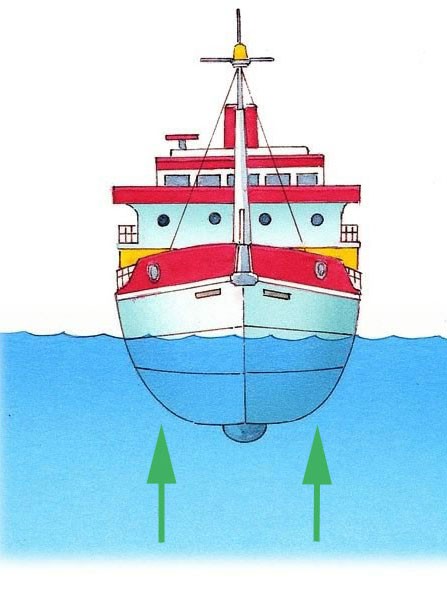
To design a marine vessel, it is very difficult to achieve a dynamic similarity for a vessel partially submerged; On the one hand, it is affected by the air forces above it. On the other hand, it is affected by the hydrodynamic force of the air below it. In addition, the motion of the waves between the air and water interfaces also affects its performance. The scaling necessities for each of these phenomena are different, so models cannot completely replicate what happens to an actual vessel. But, it can be done for an aircraft or submarine well, as each of these two works fully within one medium.

Read More on Linquip

An Easy Guideline to How to Use a Refractometer
How to Use and Read a Hydrometer: Your Concise But Complete Guide

Dimensional Analysis

In engineering and science, dimensional analysis involves identifying the base quantities of different physical quantities (such as length, time, mass, and electric current) and units of measure (such as kilometers and kilograms) and tracking these dimensions to make calculations or comparisons.

Every equation or inequality must have identical dimensions on its left and right sides. This property is known as dimensional homogeneity. Checking for this simple rule is a fundamental step of dimensional analysis.

Many parameters in physics and engineering are represented as a concrete number (a numerical value and a related dimensional unit). A quantity is usually expressed in terms of some other quantities. As a familiar example, the corresponding unit for speed is a combination of length and time (e.g., measured in meters per second). Other relations can include multiplication (often shown by a centered dot), powers (like m², square meters), or their combinations.

A set of base units for a measurement system is a chosen set of units that none of them can be expressed in terms of other ones, and all the remaining units can be expressed based on their combinations. For instance, units of length and time are generally selected as base units. Therefore, the volume of a system can be measured with the base units of length (m³).

In dimensional analysis, no physical dimension is assigned to a dimensionless quantity. It is also called a pure, bare, or scalar quantity. In fact, it is a quantity of dimension one, with a corresponding unit of one (1) in the SI, which is not explicitly demonstrated.

Buckingham π Theorem

The Buckingham π theorem shows that the validity of the laws of physics is not dependent on a particular unit system. The implication of this theorem is that any law of physics can be represented as an identity that contains only dimensionless combinations of the variables associated by law; for example, volume and pressure are inversely related by Boyle’s Law.

If the values of dimensionless combinations change with the systems of units, the equation will not be an identity, and the Buckingham theorem will not be stable. This theorem helps to find a set of independent dimensionless quantities. Suppose that there are a certain number (n) of variables in a physical problem, including m independent dimensions. So, the number of independent, dimensionless quantities is:

$p=n-m$

If we show each of the dimensionless groups with π_i, the final equation is obtained as follows:

${\pi }_1=f({\pi }_2,\ {\pi }_3,\dots ,{\pi }_{n-m})$

The π groups are independent of each other. For experimental purposes, different systems that have the same dimensionless quantities are equivalent.

Example of Buckingham π Theorem Application

Consider that we want to find the effect of the variables d, l, ρ, μ, and v on pressure drop (ΔP) in a channel in which a fluid is flowing.

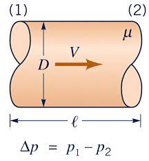
In this case, there are six variables and three base units including length (L), mass (M), and time (T). So, by Buckingham theorem:

$n-m=6-3=3$

Therefore, we will have three dimensionless groups.

For example, the dimension of ΔP is ML^-1T^-2. Based on dimensional analysis, the following dimensional groups are obtained:

${\pi }_1=\frac{l}{d}$

${\pi }_2=\frac{\mathit{\Delta}P}{\rho v^2}$

${\pi }_3=\frac{\rho vd}{\mu }$

Thus,

$\frac{\mathit{\Delta}P}{\rho v^2}=f\left(\frac{l}{d},\frac{\rho vd}{\mu }\right)$

How to Apply Similarity Laws in Fluid Dynamics

Similarity has been applied for a wide range of engineering problems and is the foundation of numerous textbook formulas and dimensionless groups. Using these formulas and quantities is easy without having to repeat the difficult process of dimensional analysis and formula derivation. Simplifying formulas (ignoring some aspects of similarity) is common and should be reviewed by an engineer for each application.

Similarity can be applied to predict the performance of a new design according to data existing from a similar design. Another use of similarity is to investigate the validation of computer simulations to reduce the need for all physical models together.

The similarity is also applicable to substitute the working fluid with a different test fluid. For example, wind tunnels have difficulty with air liquefying in certain conditions, so sometimes helium can be used instead. Moreover, dangerous or expensive fluids may not be tested in some cases, and they can be carried out in a more convenient substitute.

Suppose we want to apply similarity laws to a model whose dimensional analysis is described in the example above. Two of the three dimensionless groups obtained in this dimensional analysis include the Reynolds number and the pressure coefficient. That’s mean:

$Re=\frac{\rho vd}{\mu }$

$C_p=\frac{\mathit{\Delta}P}{\rho v^2}$

Since the dimensionless groups stay constant for both the test and the actual application, using similarity laws, we can find the force developed in the actual case (indicated by index a) based on the measured force in the model test (represented by index m).

$Re_m=Re_a$

or,

$\frac{{\rho }_mv_md_m}{{\mu }_m}=\frac{{\rho }_av_ad_a}{{\mu }_a}$

Thus,

$\frac{v_m}{v_a}=\left(\frac{{\rho }_a}{{\rho }_m}\right)\times \left(\frac{d_a}{d_m}\right)\times \left(\frac{{\mu }_m}{{\mu }_a}\right)$

Using the pressure coefficient and the following equation for calculating the pressure along the channel, the process of applying similarity laws for force measurement can be completed.

$F=\mathit{\Delta}P\ L^2$

Therefore,

$F_a=F_m\times \left(\frac{{\rho }_a}{{\rho }_m}\right)\times {\left(\frac{L_a}{L_m}\right)}^2\times {\left(\frac{v_a}{v_m}\right)}^2$

It is a simple example of the application of dimensional analysis based on similarity. However, there are some approaches to maintain kinematic similarity. Sometimes to retain the Reynolds number the same, the scaled model can utilize another fluid with different viscosity or density.

Common Dimensionless Numbers

Here are some common applications of similarity laws and associated dimensionless numbers:

Reynolds Number

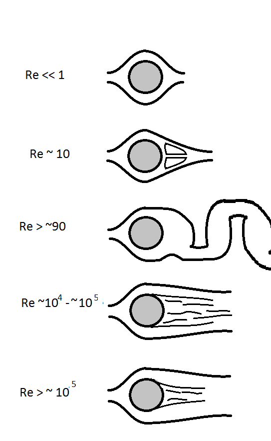
The Reynolds number (Re) helps us to identify the flow regime of a specific physical problem. The fluid flows are considered laminar (sheet-like) flow at low Reynolds numbers, but at high Reynolds numbers, the turbulence is the dominant flow regime. This dimensionless number is defined as:

$Re=\frac{\rho vL}{\mu }$

where, ρ, v, L, and μ are fluid density (kg/m³), flow velocity (m/s), characteristic length (m), and fluid viscosity (m²/s), respectively. As can be seen from the above definition, this parameter represents the ratio of inertial forces to viscous forces.

Pressure Coefficient

In fluid dynamics, the pressure coefficient describes the relative pressures in a flow field. This dimensional number is used in aerodynamics and hydrodynamics. It is a parameter for analyzing both incompressible and compressible fluids and is expressed as:

$C_p=\frac{p-p_{\infty }}{\frac{1}{2}\rho v^2_{\infty }}$

In this equation, p and p_∞ are static pressure at a given point of the flow and the free stream static pressure. Also, v_∞ is the fluid velocity of the free stream.

Froude Number

The Froude number (Fr) is defined as the ratio of the inertia to the external field (usually simply due to gravity). The Froude number is expressed by the following equation:

$Fr=\frac{u}{\sqrt{gL}}$

where u, g, and L are the local flow velocity, the local external field, a characteristic length, respectively.

The Froude number is an important parameter where a partially submerged object moves through the water.

Weber Number

The Weber number (We) is often applied where there is an interface between two different fluids, particularly for multiphase flows with curved surfaces. It is defined as:

$We=\frac{\rho v^2l}{\sigma }$

In this relation, σ is surface tension (in N/m).

The Weber number can be considered as a ratio of fluid inertia to its surface tension.

Prandtl Number

The Prandtl number (Pr) is defined as the ratio of momentum diffusivity to thermal diffusivity. This dimensionless group is expressed as:

$Pr=\frac{c_pu}{k}$

where c_p and k are fluid specific heat (J/kg.K) and thermal conductivity (W/m.K). This dimensionless number can be used to find the thermal conductivity of a gas at high temperatures, especially where it is tricky to determine experimentally due to the formation of convection flows.

Heat Capacity Ratio

In thermodynamics, the heat capacity ratio (γ) is defined as the ratio of c_p (the heat capacity at constant pressure) to c_v (the heat capacity at constant volume).

$\gamma =\frac{c_p}{c_v}$

Examples of this dimensionless number applications include thermodynamically reversible processes, especially for ideal gases, and finding the speed of sound.

Mach Number

Mach number (Ma) is a dimensionless parameter in fluid dynamics which is defined as the ratio of flow velocity to the local speed of sound. It is expressed as:

$Ma=\frac{u}{c}$

c is the sound speed in the medium. The Mach number depends on the gas (medium) temperature.

Strouhal Number

The Strouhal number (St) is a dimensionless number representing oscillating flow mechanisms. It is usually expressed as:

$St=\frac{fL}{u}$

In this relation, f is the frequency of vortex shedding.

Womersley Number

The Womersley number (α) is applicable in biofluid mechanics and biofluid dynamics. This dimensionless number expresses the pulsatile flow frequency in relation to viscosity. An example of its application is in scaling up the vascular system for experimental investigation. It is also significant in finding the thickness of the boundary layer to determine if entrance effects can be overlooked.

${\alpha }^2=\frac{\omega L^2}{\nu }$

In the above equation, ω is the angular frequency of oscillation.

Read More In Linquip